
A capacitor is a device that stores energy. Capacitors store energy in the form of an electric field. At its most simple, a capacitor can be little more than a pair of metal plates separated by air. As this constitutes an open circuit, DC current will not flow through a capacitor. If this simple device is connected to a DC voltage source, as shown in Figure 8.2.1 , negative charge will build up on the bottom plate while positive charge builds up on the top plate. This process will continue until the voltage across the capacitor is equal to that of the voltage source. In the process, a certain amount of electric charge will have accumulated on the plates. 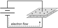 Figure 8.2.1 : Basic capacitor with voltage source. The ability of this device to store charge with regard to the voltage appearing across it is called capacitance. Its symbol is C and it has units of farads (F), in honor of Michael Faraday, a 19th century English scientist who did early work in electromagnetism. By definition, if a total charge of 1 coulomb is associated with a potential of 1 volt across the plates, then the capacitance is 1 farad. \[1 \text < farad >\equiv 1 \text < coulomb >/ 1 \text < volt>\label \] or more generally, \[C = \frac \label \] Where \(C\) is the capacitance in farads, \(Q\) is the charge in coulombs, \(V\) is the voltage in volts. From Equation \ref we can see that, for any given voltage, the greater the capacitance, the greater the amount of charge that can be stored. We can also see that, given a certain size capacitor, the greater the voltage, the greater the charge that is stored. These observations relate directly to the amount of energy that can be stored in a capacitor. Unsurprisingly, the energy stored in capacitor is proportional to the capacitance. It is also proportional to the square of the voltage across the capacitor. \[W = \frac CV^2 \label \] Where \(W\) is the energy in joules, \(C\) is the capacitance in farads, \(V\) is the voltage in volts. The basic capacitor consists of two conducting plates separated by an insulator, or dielectric. This material can be air or made from a variety of different materials such as plastics and ceramics. This is depicted in Figure 8.2.2 .
 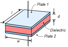 Figure 8.2.2 : Components of a generic capacitor. For practical capacitors, the plates may be stacked alternately or even made of foil and formed into a rolled tube. However it is constructed, the characteristics of the dielectric will play a major role in the performance of the device, as we shall see. In general, capacitance increases directly with plate area, \(A\), and inversely with plate separation distance, \(d\). Further, it is also proportional to a physical characteristic of the dielectric; the permittivity, \(\varepsilon\). Thus, capacitance is equal to: \[C = \varepsilon \frac \label \] Where \(C\) is the capacitance in farads, \(A\) is the plate area in square meters, \(d\) is the plate separation distance in meters, \(\varepsilon\) is permittivity of the dielectric between the plates. It should be noted that the effective plate area is somewhat larger than the precise physical area of the plates. This is due to a phenomenon called fringing. Essentially, the electric field lines bulge outward at the plate edges rather than maintain uniform parallel orientation. This is illustrated in Figure 8.2.3
  Figure 8.2.3 : Capacitor electric field with fringing. From Equation \ref it is obvious that the permittivity of the dielectric plays a major role in determining the volumetric efficiency of the capacitor, in other words, the amount of capacitance that can be packed into a given sized component. Some dielectrics are notably more efficient than others. To make comparisons easier, relative permittivity is often used, that is, the ratio of the dielectric's permittivity to that of a vacuum, \(\varepsilon_0\). A table of relative permittivity for a variety of dielectrics is shown in Table 8.2.1 . A number of common dielectrics, such as various poly plastic films and mica, exhibit permittivities two to six times that of air, but there are also ceramic dielectrics whose dielectrics are hundreds to thousands of times that of air.
| Material | Relative permittivity, \(\varepsilon_r = \varepsilon /\varepsilon_0\) |
|---|---|
| Vacuum | 1 (\(\varepsilon_0\) =8.85E−12 farads/meter) |
| Air | 1.00058986 (at STP) |
| PTFE/Teflon | 2.1 |
| Polyethylene/XLPE | 2.25 |
| Polyimide | 3.4 |
| Polypropylene | 2.2-2.36 |
| Polystyrene | 2.4-2.7 |
| Polyester (Mylar) | 3.1 |
| Paper | 1.4 |
| Mica | 3-6 |
| Silicon dioxide | 3.9 |
| Rubber | 7 |
| Diamond | 5.5-10 |
| Silicon | 11.68 |
| Titanium dioxide | 86-173 |
| Strontium titanate | 310 |
| Calcium copper titanate | >250,000 |
At quick glance, it might seem that choosing the dielectric with the highest permittivity would be the best choice but this is not necessarily the case. There are several other factors that go into this decision including temperature stability, leakage resistance (effective parallel resistance), ESR (equivalent series resistance) and breakdown strength. For an ideal capacitor, leakage resistance would be infinite and ESR would be zero. Unlike resistors, capacitors do not have maximum power dissipation ratings. Instead, they have maximum voltage ratings. The breakdown strength of the dielectric will set an upper limit on how large of a voltage may be placed across a capacitor before it is damaged. Breakdown strength is measured in volts per unit distance, thus, the closer the plates, the less voltage the capacitor can withstand. For example, halving the plate distance doubles the capacitance but also halves its voltage rating. Table 8.2.2 lists the breakdown strengths of a variety of different dielectrics. Comparing the tables of Tables 8.2.1 and 8.2.2 hints at the complexity of the situation. For instance, consider polystyrene versus polypropylene. Polystyrene offers modestly increased permittivity yet polypropylene has a considerable advantage in terms of breakdown strength. As a consequence, the plates can be placed much closer together when using polypropylene while achieving the same voltage rating as a capacitor using polystyrene. Therefore, the polypropylene capacitor will require less volume for the same capacitance. As an added benefit, polypropylene exhibits high temperature stability and low moisture absorption, among other characteristics. Comparing polypropylene to polyester, we find that polyester's improved permittivity along with a similar breakdown strength yields improved volumetric efficiency over polypropylene. Unfortunately, polyester suffers from greater temperature dependence.
| Substance | Breakdown Strength (kV/mm) |
|---|---|
| Air | 3.0 |
| Borosilicate glass | 20-40 |
| PTFE (Teflon, insulating film) | 60-173 |
| Polyethylene | 19-160 |
| Polypropylene | 650 |
| Polystyrene | 19.7 |
| PEEK (Polyether ether ketone) | 23 |
| Polyester (Mylar) | 580 |
| Neoprene rubber | 15.7-26.7 |
| Distilled water | 65-70 |
| Waxed paper | 40-60 |
| Mica | 118 |
| Diamond | 2,000 |
| PZT (ceramic) | 10-25 |
Capacitors are available in a wide range of capacitance values, from just a few picofarads to well in excess of a farad, a range of over 10\(^<12>\). Unlike resistors, whose physical size relates to their power rating and not their resistance value, the physical size of a capacitor is related to both its capacitance and its voltage rating (a consequence of Equation \ref. Modest surface mount capacitors can be quite small while the power supply filter capacitors commonly used in consumer electronics devices such as an audio amplifier can be considerably larger than a D cell battery. A sampling of capacitors is shown in Figure 8.2.4 . 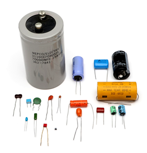 Figure 8.2.4 : A variety of capacitor styles and packages. Toward the front and left side of the photo are a variety of plastic film capacitors. The disk-shaped capacitor uses a ceramic dielectric. The small square device toward the front is a surface mount capacitor, and to its right is a teardrop-shaped tantalum capacitor, commonly used for power supply bypass applications in electronic circuits. The medium sized capacitor to the right with folded leads is a paper capacitor, at one time very popular in audio circuitry. A number of capacitors have a crimp ring at one side, including the large device with screw terminals. These are aluminum electrolytic capacitors. These devices tend to exhibit high volumetric efficiency but generally do not offer top performance in other areas such as absolute accuracy and leakage current. They usually are polarized, meaning that the leads must match the polarity of the applied voltage. Inserting them into a circuit backwards can result in catastrophic failure. The polarity is usually identified by a series of minus signs and/or a stripe that indicates the negative lead. Tantalum capacitors are also polarized but are typically denoted with a plus sign next to the positive lead. A variable capacitor used for tuning radios is shown in Figure 8.2.5 . One set of plates is fixed to the frame while an intersecting set of plates is affixed to a shaft. Rotating the shaft changes the amount of plate area that overlaps, and thus changes the capacitance.
 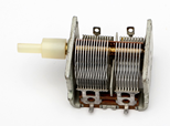 Figure 8.2.5 : A variable capacitor. For large capacitors, the capacitance value and voltage rating are usually printed directly on the case. Some capacitors use “MFD” which stands for “microfarads”. While a capacitor color code exists, rather like the resistor color code, it has generally fallen out of favor. For smaller capacitors a numeric code is used that echoes the color code. Typically it consists of a three digit number such as “152”. The first two digits are the precision portion and the third digit is the power of ten multiplier. The result is in picofarads. Thus, 152 is 1500 pf.

 Figure 8.2.6 : Capacitor schematic symbols (top-bottom): non-polarized, polarized, variable. The schematic symbols for capacitors are shown in Figure 8.2.6 . There are three symbols in wide use. The first symbol, using two parallel lines to echo the two plates, is for standard non-polarized capacitors. The second symbol represents polarized capacitors. In this variant, the positive lead is drawn with a straight line for that plate and often denoted with a plus sign. The negative terminal is drawn with a curved line. The third symbol is used for variable capacitors and is drawn with an arrow through it, rather like a rheostat.
  Figure 8.2.7 : An LCR meter, designed to read capacitance, resistance and inductance. In order to obtain accurate measurements of capacitors, an LCR meter, such as the one shown in Figure 8.2.7 , may be used. These devices are designed to measure the three common passive electrical components: resistors, capacitors and inductors 1 . Unlike a simple digital multimeter, an LCR meter can also measure the values at various AC frequencies instead of just DC, and also determine secondary characteristics such as equivalent series resistance and effective parallel leakage resistance.
A portion of a typical capacitor data sheet is shown in Figure 8.2.8 . This is for a series of through-hole style metallized film capacitors using polypropylene for the dielectric. First we see a listing of general features. For starters, we find that the capacitors use a flame retardant epoxy coating and are also RoHS compliant. We then move to a set of electrical performance specifications. For example, we see that this series is available in two variants, one rated at 800 volts DC and the other rated at 1600 volts DC. Further, tolerance is available as either \(\pm\)3% or \(\pm\)5%. Dissipation factor \((\tan \delta )\) is a measure of particular importance for AC operation and is proportional to the ESR (equivalent series resistance, ideally 0), smaller being better. The insulation resistance indicates the value of an effective parallel leakage resistance (higher is better), here, some 30,000 M\(\Omega\). Finally, we see physical size data, essential for printed circuit board layouts.
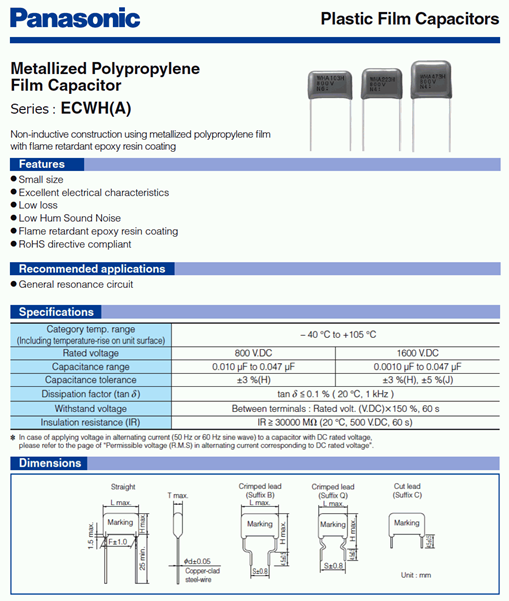
Multiple capacitors placed in series and/or parallel do not behave in the same manner as resistors. Placing capacitors in parallel increases overall plate area, and thus increases capacitance, as indicated by Equation \ref<8.4>. Therefore capacitors in parallel add in value, behaving like resistors in series. In contrast, when capacitors are placed in series, it is as if the plate distance has increased, thus decreasing capacitance. Therefore capacitors in series behave like resistors in parallel. Their value is found via the reciprocal of summed reciprocals or the product-sum rule. Figure 8.2.8 : Capacitor data sheet. Courtesy of Panasonic
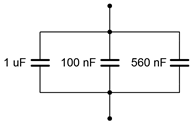
Find the equivalent capacitance of the network shown in Figure 8.2.9 . Figure 8.2.9 : Circuit for Example 8.2.1 . These capacitors are all in parallel, and thus, the equivalent value is the sum of the three capacitances: \[C_ = C_1+C_2+C_3 \nonumber \] \[C_ = 1 \mu F+100 nF+560 nF \nonumber \] \[C_ = 1.66 \mu F \nonumber \]
Find the equivalent capacitance of the network shown in Figure 8.2.10 . 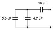 Figure 8.2.10 : Circuit for Example 8.2.2 . In this circuit, we find that the left and middle capacitors are in parallel. This combination is in series with the capacitor to the right: \[C_ = C_1+C_2 \nonumber \] \[C_ = 3.3 \mu F+4.7 \mu F \nonumber \] \[C_ = 8 \mu F \nonumber \] \[C_ = \frac< C_C_3>
 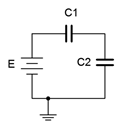 Figure 8.2.11 : A simple capacitors-only series circuit.
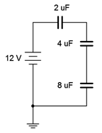
Find the voltages across the capacitors in Figure 8.2.12 . Figure 8.2.12 : Circuit for Example 8.2.3 . The first step is to determine the total capacitance. As these are in series, we can use the reciprocal rule: \[C_ = \frac<\frac + \frac + \frac> \nonumber \] \[C_ = \frac<\frac + \frac + \frac> \nonumber \] \[C_ \approx 1.143 \mu F \nonumber \] From here we determine the total charge: \[Q = V C \nonumber \] \[Q = 12 V1.143 \mu F \nonumber \] \[Q = 13.71 \mu C \nonumber \] Charge is constant across all of the series capacitors, therefore: \[V_ = \frac \nonumber \] \[V_ = \frac \nonumber \] \[V_ = 6.855V \nonumber \] \[V_ = \frac \nonumber \] \[V_ = \frac \nonumber \] \[V_ = 3.427V \nonumber \] \[V_ = \frac \nonumber \] \[V_ = \frac \nonumber \] \[V_ = 1.714V \nonumber \] The sum of the three voltages is 12 volts (within rounding error) and verifies KVL as expected.
While it may be tempting to try, do not attempt to verify the operation of Example 8.2.3 in the laboratory using a standard DMM. The reason is because the internal resistance of a typical digital voltmeter is many orders of magnitude lower than the leakage resistance of the capacitors. As a result, charge will be transferred to the meter, ruining the measurement. It would be akin to trying to measure the voltages across a string of resistors, each in excess of 100 M\(\Omega\), with a meter whose internal resistance is 1 M\(\Omega\). The meter's resistance dominates the parallel combination and causes excessive loading which ruins the measurement. A special sort of voltmeter, an electrostatic voltmeter or electrometer, is needed for these types of measurements. These are sometimes referred to as non-charge transfer meters.
The fundamental current-voltage relationship of a capacitor is not the same as that of resistors. Capacitors do not so much resist current; it is more productive to think in terms of them reacting to it. The current through a capacitor is equal to the capacitance times the rate of change of the capacitor voltage with respect to time (i.e., its slope). That is, the value of the voltage is not important, but rather how quickly the voltage is changing. Given a fixed voltage, the capacitor current is zero and thus the capacitor behaves like an open. If the voltage is changing rapidly, the current will be high and the capacitor behaves more like a short. Expressed as a formula: \[i = C \frac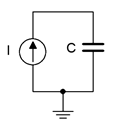 Figure 8.2.13 : Capacitor with current source.
 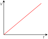 Figure 8.2.14 : Capacitor voltage versus time. As time progresses, the voltage across the capacitor increases with a positive polarity from top to bottom. With a theoretically perfect capacitor and source, this would continue forever, or until the current source was turned off. In reality, this line would either begin to deflect horizontally as the source reached its limits, or the capacitor would fail once its breakdown voltage was reached. The slope of this line is dictated by the size of the current source and the capacitance.
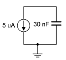
Determine the rate of change of voltage across the capacitor in the circuit of Figure 8.2.15 . Also determine the capacitor's voltage 10 milliseconds after power is switched on. Figure 8.2.15 : Circuit for Example 8.2.4 . First, note the direction of the current source. This will produce a negative voltage across the capacitor from top to bottom. The rate of change is: \[\frac = \frac \nonumber \] \[\frac = \frac \nonumber \] \[\frac \approx −166.7 \text < volts per second>\nonumber \] Thus, for every second, the voltage rises another −166.7 volts. Assuming it is completely uncharged when power is applied, after 10 milliseconds it will have risen to −166.7 V/s times 10 ms, or −1.667 volts. Equation \ref provides considerable insight into the behavior of capacitors. As just noted, if a capacitor is driven by a fixed current source, the voltage across it rises at the constant rate of \(i/C\). There is a limit to how quickly the voltage across the capacitor can change. An instantaneous change means that \(dv/dt\) is infinite, and thus, the current driving the capacitor would also have to be infinite (an impossibility). This is not an issue with resistors, which obey Ohm's law, but it is a limitation of capacitors. Therefore we can state a particularly important characteristic of capacitors: \[\text \label \] This observation will be key to understanding the operation of capacitors in DC circuits.
This page titled 8.2: Capacitance and Capacitors is shared under a CC BY-NC-SA 4.0 license and was authored, remixed, and/or curated by James M. Fiore via source content that was edited to the style and standards of the LibreTexts platform.